In July 2020, Microsoft introduced around 50 new DAX functions into Power BI. These functions are similar to those found in Excel, so some users will already be familiar with them. For those who do not have experience with these features, we aim to go through them in a series of DAX Finance articles to help you understand what they do and how to use them.
The first instalment of the DAX Finance series will introduce the depreciation functions. Note that for all of the depreciation functions, the return value is for a specified period(s) only. Generating accumulated depreciation and other derivative values is easy, but requires additional steps.
The following functions are regularly used in financial/ accounting analysis and reports.
- DB() – Fixed declining balance
- DDB() – Double-declining balance/ other
- SLN() – Straight Line
- SYD() – Sum-of-years digit
Data
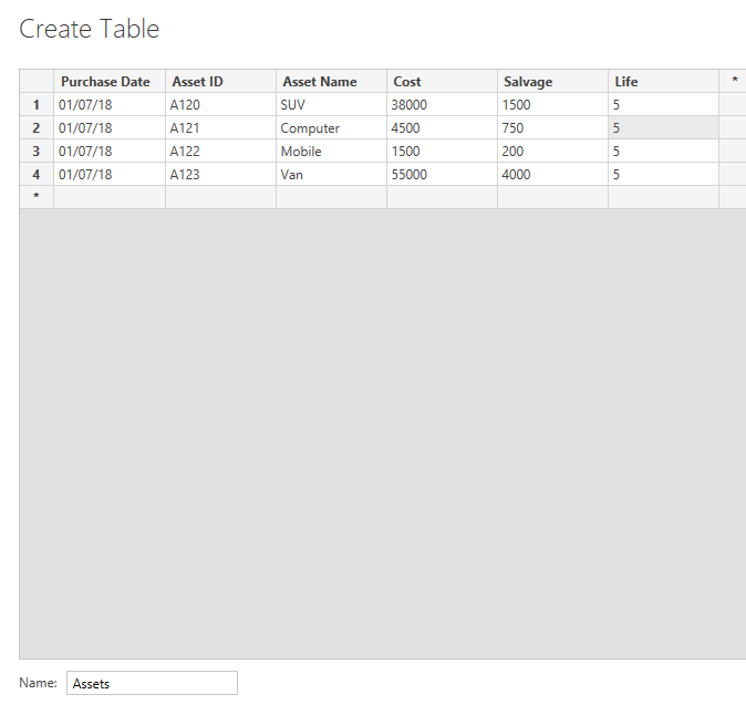
To create these examples, we will enter some data into a table.
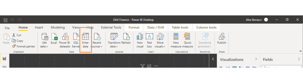
Enter the below information, name the table “Assets” and load it in.
DAX Finance Function: DB()
DB() is the fixed declining balance method which returns the depreciation of an asset for a specified period. This method is an accelerated depreciation system of recording larger depreciation expenses during the earlier years of an asset’s useful life and smaller depreciation amounts at the end of the asset’s life.
This technique is quite often used for assets such as computers, mobile phones, laptops and other high-technology products that become obsolete quickly due to newer models being released.
This method is the opposite of the straight-line depreciation method, which is more suitable for assets that drop in value at a regular rate over their lifetime.
DB uses the following formulas to calculate depreciation for a period:
- Depreciation Rate = 1 – [(Salvage / Cost)^(1 / life)]
- Depreciation for any period = (Original Costs – Total Depreciation form Prior Periods) * Depreciation Rate
- When the first period is not a full 12 months, depreciation for the first and last periods are special cases, where the number of months is used to calculate the fractional values.
- Depreciation for the first period = Cost * Rate * Months / 12
- Depreciation for the last period = ((Cost – Total Depreciation from prior periods) * Rate * (12- Months)) / 12
Syntax in Power BI
Depreciation = DB( <cost>, <salvage>, <life>, <period> [, <month> ] )
| Parameter | Attributes | Description |
|---|---|---|
| Cost | The cost of the asset | |
| Salvage | Value at end of depreciation | |
| Life | No. of periods over which asset is depreciated | |
| Period | The period you want to calculate the depreciation. Must be same units as life | |
| Month | Optional | The number of months in first year (if omitted, 12 months is assumed) |
Example
John bought a computer which was put on the company’s books at $3,000, with a salvage value of $750 and a life of 4 years.
Make sure you select New Column for the DB() function.
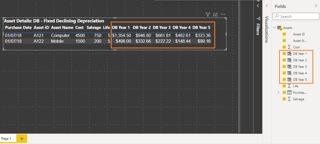
The function will appear as below.
| Calculation Name | Calculation Syntax |
|---|---|
| DB Year 1 |
DB Year 1 = DB( Assets[Cost], Assets[Salvage], Assets[Life], 1 ) |
| DB Year 2 |
DB Year 2 = DB( Assets[Cost], Assets[Salvage], Assets[Life], 2 ) |
| DB Year 3 |
DB Year 3 = DB( Assets[Cost], Assets[Salvage], Assets[Life], 3 ) |
| DB Year 4 |
DB Year 4 = DB( Assets[Cost], Assets[Salvage], Assets[Life], 4 ) |
| DB Year 5 |
DB Year 5 = DB( Assets[Cost], Assets[Salvage], Assets[Life], 5 ) |
For each new calculated column for DB Year n, select the calculation and make the following format changes:
- Currency ($)
- 2 decimal places
- Don’t summarise
If an asset’s life is less than the period being calculated there will be no depreciation to assign for that year and it will show an error. Therefore, if you have multiple assets with different life spans you will need to update the calculated column to the following:
IFERROR(DB( <Cost>, <Savage>, <Life>, <Period> [, <month> ]),0).
Here, we use IFERROR to input 0 if an error occurs.
DAX Finance Function: DDB()
DDB() is the double declining balance depreciation method, aka the reducing balance method. The double declining method is an accelerated depreciation that counts as an expense more rapidly than the straight line method (outlined below). This method depreciates assets twice as fast as the traditional declining balance method.
This technique is used on assets that are likely to lose most of their value early on or become obsolete quickly. This means that the asset will have a higher depreciation value in its early life and lower depreciation in its later years.
DDB uses the following formulas to calculate depreciation for a period:
- Depreciation Rate = 2 x SLDP x BV
where:
SLDP = Straight-line depreciation percent
BV = Book value at the beginning of the period
Syntax in Power BI
Depreciation = DDB( <cost>, <salvage>, <life>, <period> [, <factor> ] )
| Parameter | Attributes | Description |
|---|---|---|
| Cost | The cost of the asset | |
| Salvage | Value at end of depreciation | |
| Life | No. of periods over which asset is depreciated | |
| Period | The period you want to calculate the depreciation. Must be same units as life | |
| Factor | Optional | The rate at which the balance declines. If omitted it is assumed to be 2 |
Example
John bought a computer which was put on the company’s books at $3,000, with a salvage value of $750 and a life of 4 years.
Make sure you select New Column when using the DDB() function.The function will appear as below.
| Calculation Name | Calculation Syntax |
|---|---|
| DDB Year 1 |
DDB Year 1 = DDB( Assets[Cost], Assets[Salvage], Assets[Life], 1 ) |
| DDB Year 2 |
DDB Year 2 = DDB( Assets[Cost], Assets[Salvage], Assets[Life], 2 ) |
| DDB Year 3 |
DDB Year 3 = DDB( Assets[Cost], Assets[Salvage], Assets[Life], 3 ) |
| DDB Year 4 |
DDB Year 4 = DDB( Assets[Cost], Assets[Salvage], Assets[Life], 4 ) |
| DDB Year 5 |
DDB Year 5 = DDB( Assets[Cost], Assets[Salvage], Assets[Life], 5 ) |
For each new calculated column for DB Year n, select the calculation and make the following format changes:
- Currency ($)
- 2 decimal places
- Don’t summarise
If an asset’s life is less than the period being calculated there will be no depreciation to assign for that year and it will show an error. Therefore, if you have multiple assets with different life spans you will need to update the calculated column to the following:
IFERROR(DDB( <Cost>, <Savage>, <Life>, <Period> [, <month> ]),0).
Here, we use IFERROR to input 0 if an error occurs.

DAX Finance Function: SLN()
SLN() is the straight line depreciation method. It calculates the value of an asset that depreciates uniformly over each period until it reaches its salvage value. It is the most common and straightforward depreciation method for allocating the cost of a capital asset. In its simplest form, we divide the cost of an asset, less its salvage value, by the useful life of the asset.
SLN uses the following formulas to calculate depreciation for a period:
- Annual Depreciation Expense = (Cost of the Asset – Salvage Value) / Useful Life of Asset
Syntax in Power BI
Depreciation = SLN( <cost>, <salvage>, <life> )
| Parameter | Attributes | Description |
|---|---|---|
| Cost | The cost of the asset | |
| Salvage | Value at end of depreciation | |
| Life | No. of periods over which asset is depreciated |
Example
John bought a van which was put on the company’s books at $55,000, with a salvage value of $4000 and a life of 5 years.
When using the DDB() function make sure you select New Column.
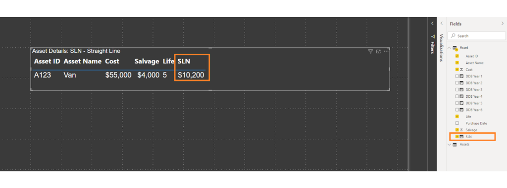
The function will appear as below.
| Calculation Name | Calculation Syntax |
|---|---|
| SLN |
SLN = SLN( Assets[Cost], Assets[Salvage], Assets[Life], ) |
For each new calculated column for DB Year n, select the calculation and make the following format changes:
- Currency ($)
- 2 decimal places
- Don’t summarise
DAX Finance Function: SYD()
SYD() is the Sum of Years Depreciation method, which is an accelerated depreciation. Quite like the double declining method, sum of years aims to depreciate a company’s assets at an accelerated rate. Companies may choose this method as it results in a larger depreciation tax shield in the first few years of the asset’s life. It is also a popular method for firms who want to write off equipment that has a high probability of becoming obsolete before salvage value is reached.
SYD uses the following formulas to calculate depreciation for a period:
- Sum of year depreciation = (Useful Life / Sum of years) * Depreciable Amount
Syntax in Power BI
Depreciation = SLN( <cost>, <salvage>, <life> , <per>)
| Parameter | Attributes | Description |
|---|---|---|
| Cost | The cost of the asset | |
| Salvage | Value at end of depreciation | |
| Life | No. of periods over which asset is depreciated | |
| Period | The period you want to calculate the depreciation. Must be same units as life |
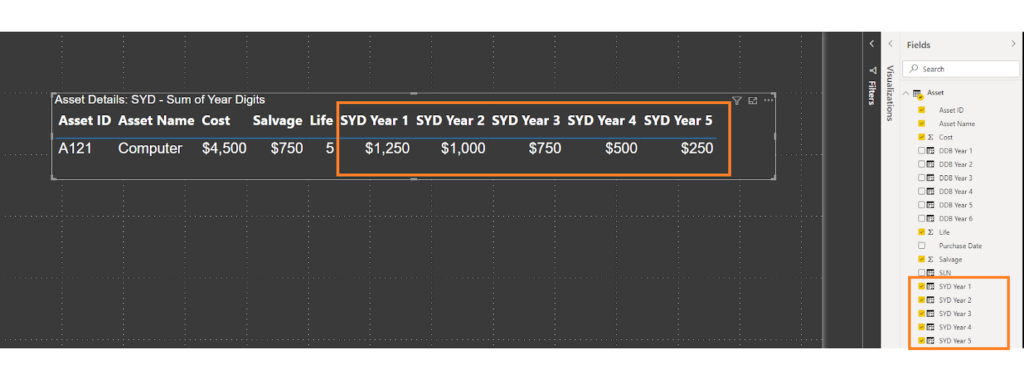
Example
John bought a computer which was put on the company’s books at $4,500, with a salvage value of $750 and a life of 5 years.
When using the DDB() function, make sure you select New Column.
The function will appear as below.
| Calculation Name | Calculation Syntax |
|---|---|
| SYD Year 1 |
SYD Year 1 = SYD( Assets[Cost], Assets[Salvage], Assets[Life], 1 ) |
| SYD Year 2 |
SYD Year 2 = SYD( Assets[Cost], Assets[Salvage], Assets[Life], 2 ) |
| SYD Year 3 |
SYD Year 3 = SYD( Assets[Cost], Assets[Salvage], Assets[Life], 3 ) |
| SYD Year 4 |
SYD Year 4 = SYD( Assets[Cost], Assets[Salvage], Assets[Life], 4 ) |
| SYD Year 5 |
SYD Year 5 = SYD( Assets[Cost], Assets[Salvage], Assets[Life], 5 ) |
For each new calculated column for DB Year n, select the calculation and make the following format changes:
- Currency ($)
- 2 decimal places
- Don’t summarise
If an asset’s life is less than the period being calculated there will be no depreciation to assign for that year and it will show an error. Therefore, if you have multiple assets with different life spans you will need to update the calculated column to the following:
IFERROR(SYD( <Cost>, <Savage>, <Life>, <Per>),0).
Here, we use IFERROR to input 0 if an error occurs.
Summary
As mentioned earlier, there are almost 50 new financial DAX functions for us to walk through. In this article we have gone through just 4 of those functions, including what they are used for and when to use them. In the next article, we will go through some more of these functions so that you eventually understand each and every one.